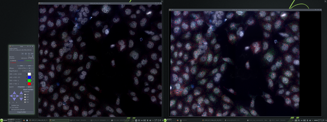
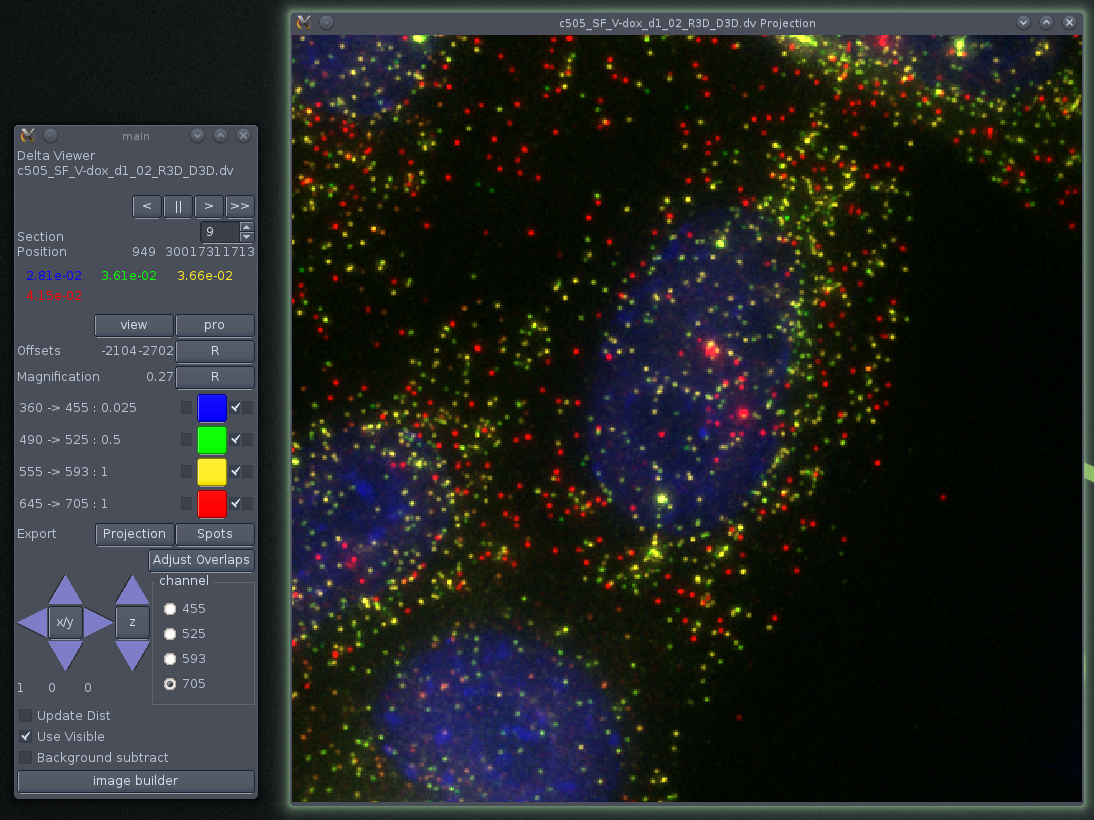
The 3 default dvReader windows. Left to right; control, optical slice and maximum intensity projection windows.

dvReader was initially just a simple viewer for looking at image stacks in the deltavision .dv format, but it has since grown to include:
However, the software remains essentially undocumented, and I usually need to consult the source code when doing anything a bit more complicated. This is an attempt to improve that situation.
The latest version can be obtained from gitorious.
dvReader works with stacks of images collected at different focal planes (z-stacks). Usually several images are collected at each focal plane using a set of channels representing different fluorophores and optionally a bright field image (DIC / phase contrast). dvReader can also handle a set of overlapping image stacks and merge these in real time without creating any intermediate files.
The 3 default dvReader windows. Left to right; control, optical slice and maximum intensity projection windows.
Although it is possible to avoid it, the application is most conveniently started from the command line. As usual, all that is required is to place the executable file, or a link to it, somewhere in the PATH. How this is done depends on the operating system used. On Macs (OSX) and Unix like systems (i.e. Linux) this is fairly straightforward, and since good terminal applications exist there is really no point in avoiding the command line. With the application in the PATH, to start the application simply do:
dvreader image_file.dv
where image_file.dv should be replaced with the name of your image file.
Starting the application on the command line makes it possible to specify several optional parameters, such as what colours to use and their respective brightness / contrast settings (see below).
The first time that you open an image set, dvReader will calculate maximum intensity projections for the image stack(s). If there are multiple stacks specified in the file and these overlap the software will also attempt to adjust the alignment of the overlapping stacks (these are usually referred to as panels). However, this function doesn't work as well as it ought to as it gets confused when overlapping areas do not contain any information (i.e. there are no objects in the overlapping area). Both the projection and the adjusted positions of the image stacks are then written to a file with the same name as the file opened, but with an additional '.info' suffix. Deleting this file is safe, but will cause dvReader to recalculate a new projection and position adjustments the next time the file is opened.
If a file contains overlapping stacks it may be necessary to also specify the '-m' option when opening the file. This specifies a margin around each image stack which is not displayed or included in any calculations. Whether or not the '-m' option is required depends on the version of softWorx (deltavision software) that was used to create the files and whether the image has been deconvolved. During deconvolution, the areas close to the borders of the image stack become distorted and no longer contain any information related to the original image. The default algorithm used by softWorx distorts all pixels lying within 32 pixels of the edges of the image stacks. In older versions of softWorx, these distorted pixels would be included in the deconvolved image stacks, and hence dvReader program needed to ignore these when merging pixels from the overlapping regions. Hence dvReader will by default ignore the areas lying within 32 pixels from the image stack edges. However newer versions of softWorx will automatically remove these pixels and adjust the positions of the resulting image stacks. For such images it's not necessary to specify a margin and in fact a 32 pixel margin may leave no overlap between neighbouring panels. In this case it's best to specify a 0 pixel margin by:
dvreader -m 0 image_file.dv
The basic dvReader interface consists of three windows: a small control window, a section viewer and a projection view. The cmd window allows the user to change the way that the channels are visualised (see below) and change certain other settings.
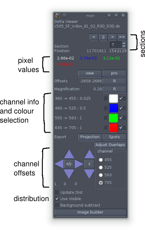
The command window.
The top of the command window tells you the current section that is displayed in the sections window and gives you some controls for changing it (though these are not usually needed). Beneath that the values for each channel at the current (or last) mouse position in the sections window are shown. Following that are controls for changing the colours used to represent the individual channels (see below).
The position and magnification of the image in the two image windows can be changed using the left and right mouse buttons. The left button moves the location of the displayed region whereas the right button changes the scale (up and right increase whereas down and left decrease magnification). Furthermore in the sections window, the mouse scroll wheel can be used to change the section that is displayed. When the window is in focus the keyboard arrow buttons can also be used to change the section.
Each focal plane of an image stack usually contains data from several channels. These are almost always simple grayscale images with the range of values being dependent on the camera and post-processing used. Most cameras used for scientific imaging have 12-bit depth; that is to say that each pixel can have a value between 0 - (212-1), although some more modern cameras have a 14 bit dynamic range. However, deconvolution of images can increase the dynamic range arbitrarily, though since the data is usually encoded as 16 bit unsigned integer values the dynamic range is unlikely to exceed 16 bits (65536 levels).
It's often stated that the human eye is only able to discertain around 256 levels of grey or a given colour, but perhaps more importantly, computer graphics specify colours using 256 levels of each of the primary colours red, green and blue. Hence to convert the raw 16 bit data in an arbitrary (but actually for deltavision quite limited) number of channels we need to perform at least two transformations.
Technically this can be done in the reverse order, but that's not very important.
The simplest way to transform a set of 16 bit values to 8 bit values is to divide all values by 256. This works, but is only reasonable if the image contains pixels throughout the 16 bit range. This is unlikely since most cameras only have 12 or 14 bits of depth. A more reasonable way is to assign values between the effective range of pixel values.
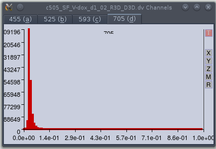
Viewing the level distributions.
Selecting the 'update dist' option in the controller window causes dvReader
to open the 'Channels' window. This has a tab for each channel containing plots of
the distributions of levels. The first time the window is opened, it will
contain empty plots; the user must load a new z-section to force the new
histogram to be displayed.
The dvReader application allows the user to specify the range for each individual channel by setting the minimum and maximum levels of the raw data; values between these extremes are simply linearly interpolated to a range between 0 and 1. To assist in setting a reasonable range, the application provides a function that plots the distribution of the raw data intensity values (after conversion from a 16 bit integers to float values). This window is displayed when the user checks the 'update dist' option in the controller window. This forces the application to obtain a full set of values for each channel each time a new section is displayed. Since this is somewhat slow it is inactive by default. After selecting this option, it is necessary to load a new section (i.e. change the z-position) to force the application to read the data. Again, this is not done by default as it can be slow when handling large image data sets.
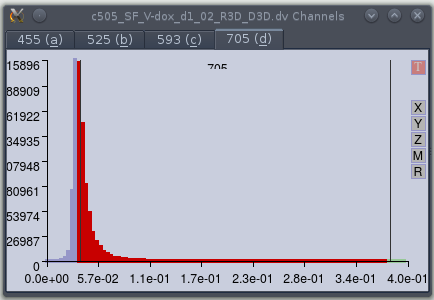
Selecting the effective range.
The user can select the effective range using the left, right and middle mouse
buttons. The left and right buttons are used to move the lower and upper thresholds
respectively, whereas the middle mouse button moves the selected range. Clicking the
'M' button (on the right) will magnify the range so that only levels within the
currently selected range are shown. In the example the plot was first magnified within
the 0-0.4 range, and then the min and maximal values selected. Areas outside of the
effective range are plotted in blue. The 'R' button restores the full range.
The range is set using the left, right and middle mouse buttons. It is also possible to magnify a region of the plot. This is frequently useful when the pixel values are concentrated at one extreme (which is very common for my experiments) and allows a much finer control of the selection.
Right-clicking the graph (without moving the cursor) will pop-up a small menu; this allows the user to save the current settings, or to load settings from a file. Saving to a file is convenient, as this can be loaded on startup via the '-r' command line switch:
dvreader -r 1.ranges image_file.dv
Where '1.ranges' is the name of the file containing the effective ranges that was saved in a previous session. There are also options to 'copy' and 'paste' the selections in the menu. However, these do not work at the time of writing and should probably be removed.
I took the code for these plots from a program (eXintegrator) I wrote much earlier for looking at microarray expression data. As a result they don't really fit very well with the rest of the application and have buttons that don't do anything. But being mainly a cosmetic issue I've not yet felt a sufficient urge to update the code.
Channel information and colour selectors
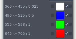
Normally the image data set will contain information from several fluorescent channels. The excitation and emission wavelengths as well as the exposure times for each channel are shown in the channel selector part of the control window next to the channel colour selector buttons.
Each channel is represented by an individual colour, with each colour defined by its red, green and blue (RGB) components. The channel RGB components are multiplied by the scaled value (see 16 bits to 8 bits above) and the final pixel RGB components are simply the sum of the channel RGB components.
The colour representing each channel can be set by clicking on the 'channel colour selectors' to the right of the channel descriptions. This will bring up a fairly standard colour selection dialog box. This allows you to set the colour by specifying either RGB or HSV (hue, saturation, value) components. Specifying the RGB components is probably the simplest option as it's easy to work out the result of combining the channels. Each component takes a value between 0 and 255 and this will be scaled to values between 0 and 1 for the colour calculations.
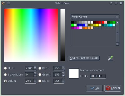
Colour chooser dialog. Nothing special
For an experiment with 3 fluorescent channels it is rather easy to choose the channel colours as one will simply assign a primary colour (i.e. red, green, or blue) to each channel. This will normally be done using the colours that most closely match the fluorophores used, but it is usually better to consider the strength of each signal and matching weak signals to colours that are easy to distinguish from a black background (i.e. red and green as opposed to blue). This will assure that all combinations of channel signals will result in unique colours that can be distinguished by eye.
For more than three channels it can be difficult to choose the channel colours as non-unique combinations will result from the blending process. If one of the channels is a non-fluorescent channel (eg. DIC) then that will normally be represented by a gray scale. As this has a neutral influence on the fluorescent channel visualisation this is not normally a problem, though it does depend on the type of data. One common method is to assign the colours that are closest to the emission colours of the fluorophores used. This is the default blended colour visualisation provided by the Deltavision software, but it's a particularly bad choice (see below) as this often makes it difficult to distinguish single signals from each other as the colours are often quite similar to each other (eg. green, yellow-red and red) and makes distinguishing specific overlaps close to impossible.
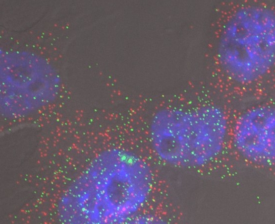
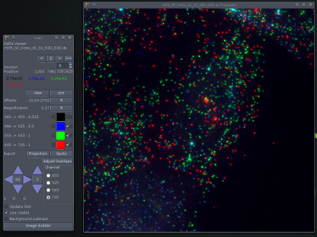
A bad selection of colours. The individual signals derive from four fluorophores, DAPI, Alexa-488, Cy3 and Cy5. These can be distinguished by the filters used in the imaging, but it is difficult to determine the origin of the individual colours in the image. This is especially so as the signals in this image are defined by specific combinations of fluorophores.
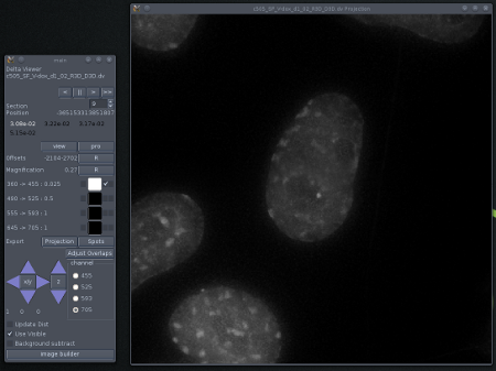
A better selection of colours. Mouse ES cells growing on a slide coated with E-cadherin and visualised by FISH against FGF4 (green) and Nanog (Red). The nuclei are stained with DAPI (blue). The grey scale indicates DIC data which gives some idea of the shape of the cells.
A better choice is usually to primary colours, plus white which will have no influence on the hue of the resulting colour. In the case above that works reasonably well as DAPI can be represented by white (i.e. grayscale). Since DAPI staining has a very different properties to the in situ signals used for the other fluorophores (punctate single mRNA molecule signals) it is easy to distinguish the DAPI and RNA signals (click here for a rather large example of this strategy).
The choice of colours can be read from a small file when starting the dvReader application. This file contains one row for each channel, with each row simply specifying the RGB components for each channel. Hence to use white, blue, green and red for DAPI, Alexa-488, Cy3 and Cy5 respectively, simply create a text file containing the following:
1   1   1
0   0   1
0   1   0
1   0   0
And if the file is called 'colors', then start the application with the '-c' switch:
dvreader -c colors image_file.dv
The channels are always internally ordered by their excitation and emission wavelengths, with an order of short to long wavelengths. This can be combined with the '-r' switch to specify the brightness and contrast of the individual channels by doing:
dvreader -c colors -r 1.ranges image_file.dv
where 'colors', '1.ranges' and 'image_file.dv' are files.
The checkboxes immediately to the right of the colour selectors indicate whether or not a channel is displayed or not. When a channel is deselected the colour of the box will turn to black and the channel will be excluded from the display (see below).
Using 3 of four channels (No DAPI)
Using only the DAPI channel