Main Window

ALERT: not up to date. Some new undescribed functionality is present

After logging in the user is confronted with the applications main window. Thiw window allows the user to access the different functions of the program through subsidiary windows (or widgets). Closing the main window quits the application.

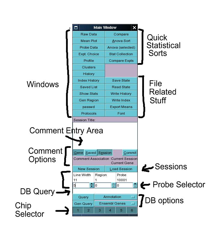
The main window contains 2 columns of buttons in addition to a text input field, a database query area and a row of chip selectors at the bottom.

Probe set selections

Almost all operations carried out by the server are carried out on the currently selected set of probes. This selection is initially made by a database query on the annotation of the probe sets, but this selection can be further modified by statistical operations. Database queries are entered onto the db query line. The text entered is then queried against the data base table selected by the table selector (see below).

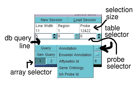
There are currently 5 different tables which hold annotation linked to probe sets.

Annotation: This contains the annotation we received from affymetrix, in addition to the annotation of associated uni-gene entries. Whereas this gives some information for most probe sets there are a number of probe sets for which this information may be incomplete or inaccurate. This annotation does not include many gene synonyms and lookups on this table are often incomplete. However, the table is reasonably small and lookups can be done quickly
Ensembl Annotation: This table contains annotation for Ensembl gene predictions. The system uses the coordinates of probe set sequence blast matches to genomic sequence in order to associate probe set identities with Ensembl genes. This allows the user to select probe-sets on the basis of the associated annotation provided by Ensembl. This will frequently return a larger number of probe sets than queries on the 'annotation' table. In addition it allows the user to make queries using things like protein family ids (as long as these are known), which have been automatically assigned by Ensembl. Note that all of the Ensembl annotation has been dumped into one huge table, and as such queries on this table may take a few seconds to complete.
Affymetrix Id: Allows probe sets to be selected by their Affymetrix ids.
Gene Ontology: This table uses a very old linkage of uni-gene id's to the GO terms. This isn't particularly useful at this time as the linkage is not particularly complete or accurate, and the entry is there primarily in order to remind me to update the linkages.
Ish Probe Id: We have performed in situ hybridisation on a number of genes linked to specific probe sets. These in-situ probes are incorporated into the database and displayed in the genomic region viewer. Probe sets associated with these in-situ probes can be selected by making queries against this table.

All queries are treated as case insensitive regular expressions, which allow the user to make complex queries using a single line. The use of regular expressions is a complex topic and will not be treated in any depth here (users are adviced to google for more information) except to highlight a few important points.

. (a dot or a period) matches any character
* matches 0 or more of the preceding character
+ matches 1 or more of the preceding character, 'hox+' does not match hox but matches hoxx and hoxxx etc..
[] matches any of the characters within the bracket, i.e. 'hox[abcd][0-9] match all instances of hox followed by a, b, c or d followed by a digit between 0 and 9.
? optional character, i.e. 'hoxb-?3' matches both hoxb3 and hoxb-3
\s matches a space (including tabs and newlines). Hence '\s+' matches one or more spaces
\S matches a non-space (opposite of preceeding)
| or, allows alternatives. 'hoxb1|hoxb2' matches both hoxb1 and hoxb2
& and, requires both terms to match. 'hox&homoedomain' requires that both hox and homeodomain are present in the record.

There's a lot more to regular expressions than this, but for the uninitiated the most important thing to remember is that '.' allows you to get all probe sets which are associated with the contents of a given table whereas '*' on its own has no meaning and will not give you anything.

After entering the query either press return or press the button underneath labelled 'Query'. The database query will then be sent to the server process will create an SQL query and pass this on to the database backend. If the 'Ensembl Annotation' table has been selected the query may take a few seconds to complete, whereas the other tables should give results within 1 or 2 seconds (though this can vary depending on the memory state of the server). A successful query will result in a new number appearing in the selection size field, the value in the probe selector being set to 0 and for the expression and annotation for the first probe set selected to be loaded by the client program and displayed in appropriate windows if open. If the query does not return any probe sets the selection size will be set to -1 and the last selected probe set will remain selected. Any further statistical queries requested (with exception of the 'Compare' function) will be carried out only on this selection. The expression of additional probe sets in the selection can be viewed by incrementing the value in 'probe selector' spin box (either by clicking the up or down arrows, entering a number directly or by selecting the spin box and using the keyboard up and down arrows).

Database queries can also be made using the genomic region mode, by selecting a table from the lower pop-up menu and pressing the 'Gen Query' button rather than the 'Query' button. This query type is made against a table containing objects with given genomic locations (such as Ensembl genes or Fantom transcripts). The server program initially gets a set of genomic regions from the query, which are then merged if they should happen to be adjacent to each other. These regions are then defined as simply as a list of genomic coordinates which are maintained by the server application. These regions can be loaded by the client application by selecting the regions using the Region spin box (the central spin box, to the left of the probe selector). When this is done the information describing that region is loaded by the client application (and displayed by the probe-data window by selecting the 'Region' toggle button at the top of probe-data window). This also causes the client application to load all probe sets associated (i.e. mapped to this region) into the index which can then be handled in the normal fashion.

The database queries only return probe sets represented by the currently selected arrays (or chips). These are selected by the toggle buttons at the bottom of the main window. Buttons 1-3 represent the MGU74Av2 chips A, B and C, buttons 4 and 5 represent the MOE430 A and B chips respectively whereas button 6 represents the second version of the MOE430 chip. Since the second version of the MOE430 chip actually represents the same probe sets as are present on MOE430 A and B chips the user may notice that the actions of these buttons are not independent. Play around with it, and work it out.. Note that the identity of the buttons is not hard-coded but is dependant on the contents of the database, so this may change depending on a given installation.

Useful probe set selection buttons

Remove probe set buttons

Towards the bottom of the window you can find a row of buttons labelled "Remove". These buttons remove probe sets from the currently selection of probe sets. The meanings are fairly self-explanatory, so do go ahead and experiment. Note that you can undo your mistakes from the "Index History" window (see about halfway down on the upper left column of buttons).

Expand by Gene

This takes the current selection of probe sets, and expands and reorders it such that probe sets are ordered by gene rather than by probe set. This can be used to select probe sets from separate array types, or simply to find all probe sets for selected genes. Play around with it to work out how it works.

All those buttons at the top of the window

The buttons in the top area of the window can be divided into three main categories:

Buttons which open additional windows which display information or allow the the specification of queries (left column)

Raw Data This opens the main expression viewing window, which displays the expression for one probe set at a time
Mean Plot This opens a window which displays the mean expression of a number of probe sets at the same time. The probe sets to be viewed are selected using the history or the saved list window (see buttons further down)
Probe Data This opens a window which displays annotation for the currently loaded probe set. The annotation includes basic annotation as well as a view of the genomic locus where the probe set matches
Samples Opens a window which allows the user to select which experiments (samples) are displayed and used in statistical analyses. Also allows the user to reorder the default display order of the experiments.
Profile This window allows the user to specify an expression profile and instruct the server process to order probe sets by their similarity to the profile
Clusters Allows the user to perform simple k-means clustering
Index History This window contains the details of the last 20 selections performed. It allows the reloading of boolean combinations of past selections
Show Stats Opens a window which displays statistics which have been requested by the user (see details for profile, and stats button below)
Gen Region Opens a window which allows the user to download and view information from a specified genomic region (currently this is broken)
passwd Opens a window which allows the user to change the password. This window also allows the administrator to create new users
Compare Samples Opens a window which allows the user to compare the different experiments (samples) in the database to each other on the basis of the currently selected probe sets.

Buttons which perform statistical queries directly (top right)

Compare This button instructs the server to compare the expression pattern of the current probe set against all other probe sets available in the database. This function does not respect the current probe set selection. The comparison algorithm calculates the euclidean distances of individual probe pair profiles against individual probe pair profiles and takes the mean value of the distances. This means that a comparison of two probe sets containing 16 probe pairs each requires the calculation of 256 individual distances of which the mean is taken. This procedure was chosen mainly because it should be ridiculously slow (to get a feeling for what one can get away with). It has one strange property for a comparison algorithm in that a probe set is not necessarily most similar to itself. It should probably be replaced with a more reasonable algorithm at some point in the futre.
Anova Sort This sorts the currently selected probe sets by the anova score calculated as the variance within individual probe pairs over the variance between samples. This button causes the calculation to be done for all experiments (samples) regardless of the current experiment selection. Dont use this if you have complex sets of data using different types of arrays, as the results can be a bit confusing.
Anova Select As above, but uses only the currenlt selection of experiments for the calculation
Stat Collection Requests the server to calculate three different statistics for the currently selected probe sets. The statistics are, Anova Score, intra euclidean distance and coefficient of variance. The intra-euclidean distance statistic doesn't really appear to work very well, so generally this can be ignored. The statistics once calculated are passed on to the Statistics window which can be opened by pressing the 'Show Stats' button in the left button field (see above).
Compare Expts This button is misplaced, see above for a description.

Buttons which perform file related tasks (bottom right)

Save State This writes the current probe set index, current probe position and any saved probe sets to a file. This file contains probe set indices and can be used to recreate the current selections at a later stage (except for ..)
Read State Reads a file created by the Save state function, or any file following the appropriate semantics. This can be useful if one wishes to load a set of probe sets selected by external analysis of the data (requires a little bit of scripting, and direct access to the underlying database).
Write History Somewhat misnamed function. Saves expression patterns saved in the 'Saved List' to a directory. This function creates a directory (specified by the user) into which it creates image files of the expression patterns of the saved list along with an html file (called index.html) which allows these to be viewed along with some probe set annotation (could do with some further development).
Write Index. As above, but for the currently selected index. Don't do this with an index of more than a 100 or so (anyway pointless) as all of the data has to be downloaded from the server and this will take some considerable time.
Export Means. Writes mean expression (1 value for each probe-set / sample rather than 16) values to a tab delimited file format. This uses the means of normalised expression profiles (see 'Raw Data' window).
Font. Not file related, guess what it does.

Comments, user annotation and sessions

The text input field below the top area of buttons is used for entering comments or user annotation into the database. The area immediately beneath this contains 3 toggle buttons which control what the comment becomes associated with, in addition to a button which commits the comment to the database. A comment can be associated with a group of probe-sets, an individual probe-set or a user session (described later) as well as combinations of the above. To associate comments with the current probe set, make sure that the 'Gene' button is toggled (appears pressed down), to associate the current probe set with the current session, toggle the session button. Additionally it is possible to associate a comment with a group of probe-sets by first saving these into the saved list (done from the history window). The mechanisms for entering comments are somewhat more complicated than they should be, and I hope to find the time to sort this out one of these days.

Lists of genes can be stored in the database, by using the above mentioned procedures. Thes lists are referred to as sessions. New sessions can be created using the 'New Session' button, and old sessions can be accessed using the 'Load Sessions' button. These are described in more detail here.